May-8-2015 Lab 16: Angular Acceleration

Part 1 : We want to apply a known torque to an object that can rotate, and measure the angular acceleration. we can find a measured value for the moment of inertia. 





this is set up to do this lab. we can use it to measure the angular acceleration. 
































1.Before we start the experiment, we measured each of the following:


2. we plug the power supply into the Pasco ratational sensor. there is a cable with the yellow paint or tape, connect only that cable to the Lab Pro at Dig/Sonic 1, so the computer could read the top disk.

3. Set up the computer. Open Logger Pro. Choose Rotary Motion. there are 200 marks on our top disk, so we need to set the Equation in the Sensor Settings to counts per rotation. when we collect data, we can see graphs of angular position, angular velocity and angular acceleration vs. time. However, the graph of angular acceleration vs. time is useless due to the poor timing resolution if the sensors.

4. Make sure the hose clamp on the bottom is open so that the bottom disk will rotate independently of the top disk when the drop pin is in place.

5. Turn on the compressed air so that the disks can rotate separately. Set the disks spinning freely to test the equipment. 

6. With the string wrapped around the torque pulley and the hanging mass at its highest point, start the measurements and release the mass. 

EXPTS 1,2, and 3: we are going to look at the effect of changing the hanging mass(25 g, 50 g, 75 g). 

Here is graph of Expt 1: 



Here is graph of Expt 2 :

Here is graph of Expt 3: 

For Expt 1 and 4, we are going to look at the effect of changing the radius and which the hanging mass exerts a torque (small torque pulley, Large torque pulley). 

Here is graph of Expt 4: 

For Expt 4, 5, and 6, we are going to look at effect of changing the rotating mass(top steel, top aluminum, top steel + bottom steel).

Here is graph of Expt 5: 

Here is graph of Expt 6: 

After linear fit those angular velocity vs. time graphs, we can know the angular acceleration up and down for each Expt.

Then we calculated  the average of angular acceleration of each Expt, we write down all data we collected into a form:

From those graphs, the we could know the angular acceleration up is always bigger than the angular acceleration down because we cant ignore some frictional torque in the system. So, When the hanging mass is going down, the net torque is equal to torque mass - torque friction , so angular acceleration down is smaller than the real.

Conclusion: 
From this form, we could see For Expt 1,2, and 3, when the mass of hanging mass is increasing, the angular acceleration is increasing.
For Expt 1 and 4, with same hanging mass, when radius of torque pulley is increasing, the angular acceleration is increasing.
For Expt 4, 5, and 6, with same hanging mass, when the rotating mass is increasing, the angular acceleration is decreasing.


Part 2:

For this part, we can use our data (which from part 1) to determine the moment of inertia of each of disks.

Purpose:
we want to work out the torque of friction, Because there is some frictional torque in the system, the angular acceleration of system when mass is descending is not the same as when it is ascending.

First, let's call the counterclockwise direction of rotation positive and clockwise direction of rotation negative. Newton's second law would lead us to predict that:

Here is calculation for Expt 1: 

By formula, we calculated the inertia of disk is 0.0025556 kg*m^2



By measurement, we got the inertia of disk is 0.0026563 kg*m^2


Comparing the moment of inertia by using formula and by using measurement, the uncertainty is 3.8%. 





by formula, we can get the value of frictional torque = 0.000178 N*m 











Here is calculation for Expt 2: 

By formula, we calculated the inertia of disk is 0.0026553 kg*m^2



By measurement, we got the inertia of disk is 0.0026563 kg*m^2



Comparing the moment of inertia by using formula and by using measurement, the uncertainty is 0.3%.




by formula, we can get the value of frictional torque = 0.0002639 N*m 












Here is calculation for Expt 3: 

By formula, we calculated the
inertia of disk is 0.0026653 kg*m^2



By measurement, we got the inertia of disk is 0.0026563 kg*m^2



Comparing the moment of inertia by using formula and by using measurement, the uncertainty is 0.339%.




by formula, we can get the value of frictional torque = 0.000265 N*m 

Here is calculation for Expt 4: 

By formula, we calculated the
inertia of disk is 0.002614 kg*m^2



By measurement, we got the inertia of disk is 0.0026563 kg*m^2



Comparing the moment of inertia by using formula and by using measurement, the uncertainty is 1.59%.




by formula, we can get the value of frictional torque = 0.000341 N*m 

Here is calculation for Expt 5: 

By formula, we calculated the
inertia of disk is 0.0009133 kg*m^2



By measurement, we got the inertia of disk is 0.0009102 kg*m^2



Comparing the moment of inertia by using formula and by using measurement, the uncertainty is 0.35%.




by formula, we can get the value of frictional torque = 0.0003566 N*m 

Here is calculation for Expt 6: 

By formula, we calculated the
inertia of disk is 0.005152 kg*m^2



By measurement, we got the inertia of disk is 0.005313 kg*m^2



Comparing the moment of inertia by using formula and by using measurement, the uncertainty is 3.41%.




by formula, we can get the value of frictional torque = 0.0002868 N*m 

Conclusion :

For Expt 2, 3, and 5, their uncertainties that we calculated are very small(under 1%), we could say our predict values of inertia of disk is very close to the values of inertia of disk we measured.
However, for Expt 1, 4, and 6, their uncertainties are little bit big. our data, like radius and weight, we may made some mistakes for measuring them. and, during the disk spinning, top disk may not rotate independently with bottom disk.

May-7-2015 Lab 15: Inelastic Collision

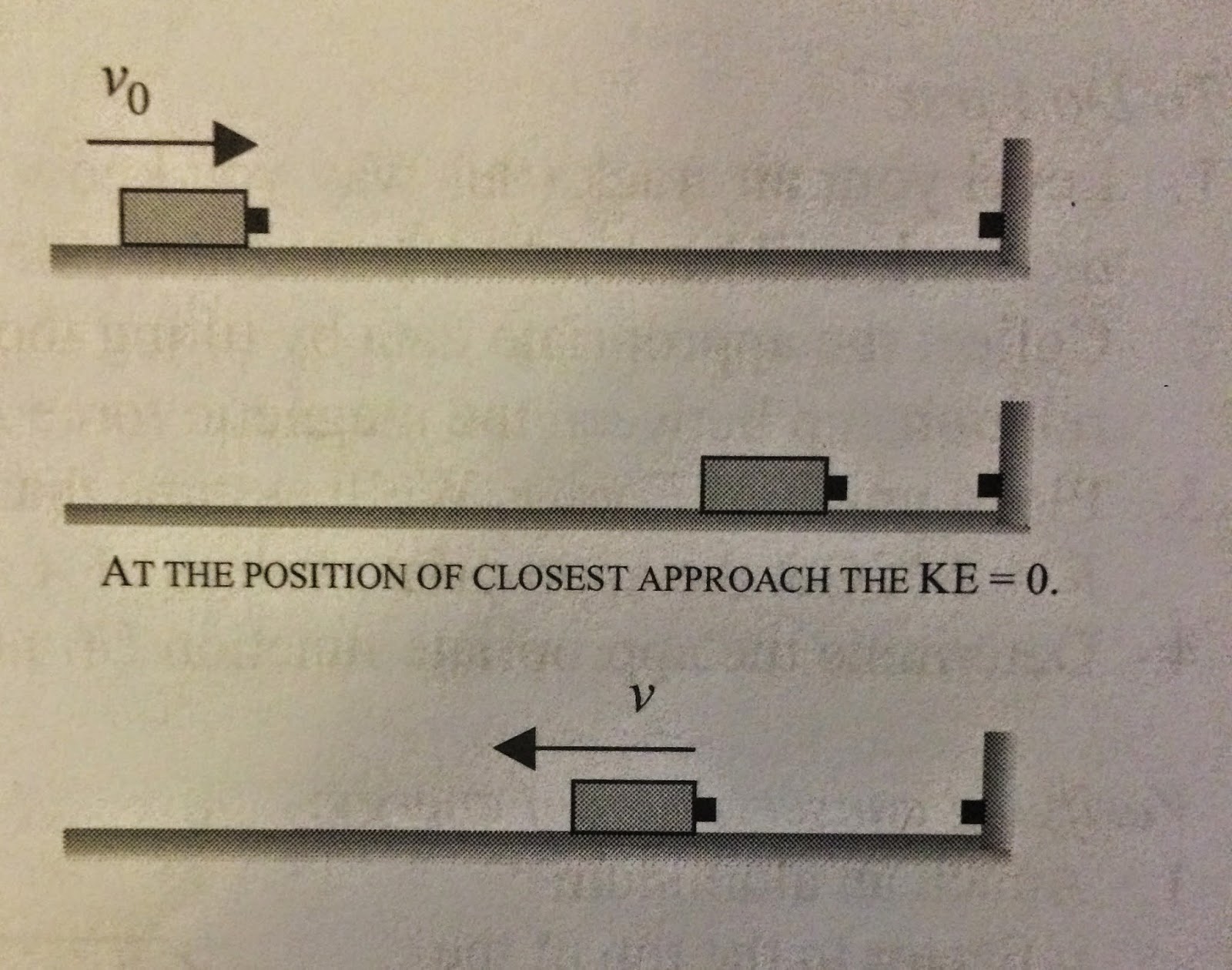
Purpose :  work out the initial speed of the small ball and its speed of uncertainty by using a small ball to hit the holder from the machine which like the picture.

set up:


Using this machine, we could give the small ball a initial speed, and the holder will hold the ball (which means they will stick together) when the ball hit the holder .  In addition, there is a red rod that will show us the highest position and angle of the holder.

After we collect all of data we need, we could calculate the initial speed of the ball by Laws of conservation of momentum and energy conservation.



Put the holder at the initial position, and put ball into the machine. then push the button, the ball will shoot out and hit the holder.

there is the graph after the ball and holder stick together, and the data we measured:

we measured the mass of ball M(ball) = 7.63 g +- 0.1 g

M(block) = 80.9 g +- 0.1 g

the changing degree of the holder:     θ = 17.5 degrees +- 0.5 degrees

the length of the string L = 0.201 m +- 0.001 m







after the ball and holder stick together, the velocity will change. so we need to know the velocity when ball and holder stick V(total) which we could calculated it by using law of  energy conservation,  Then we could know the initial speed of the ball V(ball) of ball by using law of momentum conservation.  Here is calculation:  

there is calculation to find ball's uncertainty of initial speed:

Conclusion :

For this lab, we measured the length of string, mass of ball and holder, and we collected the changing of degree of the holder after we shot the ball. Then we used the laws of conservation of momentum and energy conservation to work out the initial speed of the ball is 4.9545 m/s, and its uncertainty is only 3.22%. that's mean Our result is pretty good.

May-6-2015 Lab 14: Collisions in two dimensions

the Purpose of this lab: look at a two-dimensional collision and determine if momentum and energy are conserved.

           -steel ball with steel ball

           -steel ball with aluminum ball

we got the experiment equipment like the picture.

Open the program, go to set up the camera by following those steps:

Camera settings (continued):

Lab setup:

Before we start the lab, we need to level the table first. 

Then gently set the stationary ball on the leveled glass table. 

Aim the rolling ball so that it hits the side of the stationary ball. 

The balls should ideally roll of at some decent angle from one another. 

after we got the video of two ball collision, we need to do something on the video: Grab the point which two ball just collided to rotate the axes, set origin and add point series for the way of ball path. 

First, we do steel ball collide with steel ball. what we got from the experiment is : 

We measured the mass of steel ball m(sb) = 0.07 kg.

after linear fit all of those point, we could have the velocities at x-axis (horizontal with initial velocity) and y-axis(vertical with initial velocity ) before and after two ball collision. 

Here is the calculation:

before two ball collision:

we got the velocity at x-axis V(x) = 0.8474 m/s (which is the slope of green points) and V(y) = 0.0062 m/s (which is the slope of red points) of first steel ball. 

second ball is at rest.

from the data we collected, we calculated the momentum of two balls before collision p(x) = 0.059 kg*m/s and the momentum of two balls after collision p(2x) = 0.056 kg*m/s at x-axis. 

in addition, we calculated the momentum of two balls before collision p(y) = 0.004 kg*m/s and the momentum of two balls after collision p(2y) = -0.003 kg*m/s at y-axis. 

here is the calculation of energy:

conclusions:  p(x) and p(2x) are pretty close, p(y) and p(2y) are also very close, so we could say the momentum is conserved in this two steel balls of two-dimensional collision. 

however, the initial kinetic energy KE(i) is bigger than final kinetic energy KE(f). there were some energy lost from this collision. so we could say the energy is not conserved in this two steel balls of two-dimensional collision.

Right now, we do the steel ball collide with aluminum ball. we measured the mass of aluminum ball m(ab) = 0.02 kg. there is what we got from the experiment:

after linear fit all of those point, we could have the velocities at x-axis (horizontal with initial velocity) and y-axis(vertical with initial velocity ) before and after two balls collision.

Here is the calculation:

before two ball collision:

we got the velocity at x-axis V(x) = 0.6071 m/s (which is the slope of green points) and V(y) = -0.0034 m/s (which is the slope of red points) of the steel ball. 

the aluminum ball is at rest.

from the data we collected, we calculated the momentum of two balls before collision p(x) = 0.0425 kg*m/s and the momentum of two balls after collision p(2x) = 0.0444 kg*m/s at x-axis. 

we calculated the momentum of two balls before collision p(y) = -0.00024 kg*m/s and the momentum of two balls after collision p(2y) = 0.0016 kg*m/s at y-axis. 

here is the calculation of energy: 

conclusions:  p(x) and p(2x) are pretty close, p(y) and p(2y) are also very close, so we could say the momentum is conserved in this two steel balls of two-dimensional collision. 

however, the initial kinetic energy KE(i) is smaller than final kinetic energy KE(f). there were some energy lost from this collision. so we could say the energy is not conserved in this two steel balls of two-dimensional collision.

Apr-19-2015 Lab 13: Impulse-Momentum activity

Introduction: Impulse combines the applied force and the time interval over which that force acts.

For a constant force F acting over a time interval t, the impulse J = F*t.  

However, if the force is not constant, we can still calculate the impulse as the area under the force vs. time graph. 

The impulse-momentum theorem states that the amount of momentum change for the moving cart is equal to the amount of the net impulse acting on the cart.

our purpose of this lab is to test this idea.

EXPT 1: Observing Collision forces that change with time.

First, set up like the picture: 

we could measure the impulse acting on the cart by taking the area under the force vs time graph for the collision, and measure the change in momentum of the cart by knowing its mass and measuring its velocity before and after the collision using the motion detector. 

1. Fasten the force probe securely to the cart so that the rubber stopper extends beyond the front of the cart. set the positive direction is toward the right. 

2. set up the motion detector. be sure that the ramp is level. 

3. We measured the mass of the cart and sensor m = 0.635 kg.

4. Open the experiment file called Impulse and Momentum.cmbl, set up to record force and motion data at 50 data points per second. 

5. zero the force probe and begin graph. then give the cart a push toward the wall. 

after we did by following the steps, we got the graph:

red line is the graph of Force vs. time.

this blue line is the graph of position vs. time.

this blue line is the graph of velocity vs. time.

From this graph, after we integral the graph of force vs. time we got the area A = -0.3952. 

after we liner fit the graph of position vs. time before the collision, we got the slope m = 0.3615 which states the cart's velocity before the collision v(0) = m = 0.3615 m/s

after we liner fit the graph of position vs. time after the collision, we got the slope m = -0.2790 which states the cart's velocity after the collision v(f) = m = -0.2790 m/s

Then, we did the calculation to test that the impulse is equal to momentum or not.

we could see the impulse J = mv(f) - mv(0) = -0.4067 is very close to the area under the graph of   force vs. time which states the momentum. 

EXPT 2 : A larger Momentum change.

this experiment is same as experiment 1 but add 200 grams of mass to our cart. m = 0.835 kg.

Repeat the experiment using a more massive cart. record the appropriate data and graphs.

red line is the graph of Force vs. time.

this blue line is the graph of position vs. time.

this blue line is the graph of velocity vs. time.

From this graph, after we integral the graph of force vs. time we got the area A = -0.6621. 

after we liner fit the graph of position vs. time before the collision, we got the slope m = 0.4435 which states the cart's velocity before the collision v(0) = m = 0.4435 m/s

after we liner fit the graph of position vs. time after the collision, we got the slope m = -0.3622 which states the cart's velocity after the collision v(f) = m = -0.3622 m/s

Then, we did the calculation to test that the impulse is equal to momentum or not.

For this experiment,  the impulse J = mv(f) - mv(0) = -0.6728 is still very close to the area under the graph of  force vs. time which states the momentum. 

EXPT 3 : Impulse-Momentum theorem in an inelastic collision.

It is also possible to examine the impulse-momentum theorem in a collision where the cart sticks to the wall and comes to rest after the collision.

leave the extra mass on cart so that its mass is the same as expt 2.  m = 0.835 kg.

we predict that the impulse is same as the nearly elastic collision. and we predict that the impulse is equal to the momentum. 

red line is the graph of Force vs. time.

this blue line is the graph of position vs. time.

this blue line is the graph of velocity vs. time.

From this graph, after we integral the graph of force vs. time we got the area A = -0.1763. 

after we liner fit the graph of position vs. time before the collision, we got the slope m = 0.22 which states the cart's velocity before the collision v(0) = m = 0.22 m/s

after the cart hits the wall, it comes to rest. v(f) = 0.

Then, we did the calculation to test that the impulse is equal to momentum or not.

For this experiment,  the impulse J = mv(f) - mv(0) = -0.1837 is still very close to the area under the graph of  force vs. time which states the momentum.

Conclusion:

For those three experiments, all of the impulses we calculated and all of the areas under the graph of  force vs. time are very close. If we could ignore some uncertainties (which like air friction,etc.), we could say that the impulse-momentum theorem can be used on those three conditions.  

Apr-19-2015 Lab 12: Magnetic Potential Energy Lab

The set up:
A frictionless cart with a strong magnet on one end approaches a fixed magnet of the same polarity:

For this lab, our goal is verify that conservation of energy applies to this system.

To do first:
we will use a glider on an air track as our cart on a frictionless surface. if we raise one end of the air track the cart will end up at some equilibrium position, where the magnetic repulsion force between the two magnets will equal the gravitational force component on the cart parallel to the track.

We measured the mass of air track m= 0.354 kg.







we measured 4 sets of data about the r and the angle between ground and the air track.

because the magnetic repulsion force between the two magnets will equal the gravitational force component on the cart parallel to the track, we got F=mg*sinθ. 

then we could calculate the force F from the θ we measured.










Open the program, we put the 4 sets of force and r into the program, then we got the graph of F vs. r. we will assume that the relationship takes the form of a power law: F = Ar^n.

After curve fit our graph, we got two equations about force F and work done U(r) which come from the interaction between the magnets:

Right now, we are verifying conservation of energy:

We measured the separation distance between the magnets d= 0.28 m.

now, we have a way to measure both the speed of the cart "velocity" and the separation between the magnets at the same time.  However, For this part, the r should be the distance between the magnet on the air track and the sensor. so that r = "position" - d.

then we set the calculated column:
PE = U(r) = 0.006754 * r^(-1.349)

KE = 1/2 * m * "velocity"^2

Total energy TE = KE + PE

Start with the cart at the far end of the track. Start the detector, then give the cart a gentle push.

after we done with experiment, we got the graph like this :

yellow line is the graph of TE vs. time


Purple line is the graph of PE vs. time


Red line is the graph of KE vs. time




Conclusion:

For this experiment, there should no any energy will lose. so the KE of air track for the time before the collision should be same as the time after the collision. However,They are not same on our graph.
From this result I think our set up may not perfect, or our separation distance may not exactly correct, or we may made some mistakes we did not know during the experiment.  This experiment requires frictionless, but we cant completely ignore the air friction. All of those things could affect the result.

Apr-18-2015. Lab 11 : Conservation of energy----Mass-spring System

For this lab, We will be looking at the energy in a vertically-oscillating mass-spring system, where the spring has a non-negligible mass.

Before we can actually to do the lab there is some preliminary stuff to work out.

assume that the gravitational PE = 0 at the ground, and that you have a spring whose top is held fixed at a height H above the ground, and the bottom of the spring is at a position y above the ground.











there is the picture show that the GPE of the spring is mg(H+y)/2 be written as m(spring)/2 *g*H + m(spring)/2 *g*y:

Now put the origin at the top of the spring and call downward the positive direction, assume that the spring has a length L, the top of the spring is held at rest but that the bottom end of the spring is moving at a speed v downward.
there is the picture show that the KE of the moving spring is 1/2 *(1/3 *m(spring))*v^2.

then set up the spring, a 50-gram mass hanger, with the motion detector on the floor. we measured the length of the spring L = 0.485 m, the mass of the spring m(spring) = 0.24 kg.

First, we need to Determining the Spring constant of the spring.

mount a table clamp with a vertical rod to the table. mount a horizontal rod to the vertical rod. Put the Force sensor on the horizontal rod with the loop of the sensor pointing downward.


place a 50-gram the mass hanger so that it is vertical and the spring is just unstretched. zero the sensor with the mass hanger in this position.






Open the program, start collecting data and slowly pull down on the 50-gram mass . then we got the graph of Force vs. position.

after we liner fit the graph, we got the slope which is the constant of spring K = -8.03 N/m .


Right now, we need To do:
      Hang 250-grams on the mass hanger. After the spring is not stretch any more, we measured the y(0) = 0.73 m.

we have expressions of KE, GPE, PE that we worked out before:

we have the mass of the spring m(spring) = 0.24 kg  ,
the constant of the spring K = -8.03 N/m,    mass of hanging M = 0.25 kg.    y(0) = 0.73 m,
△y = 0.843 - "position"(we could measure it from the sensor)
the velocity v (we could measure it from sensor).

Under the Data menu in loggerPro, we created:
the New calculated column of KE = 1/2 *(M + 1/3 *m(spring))*v^2.
the New calculated column of GPE = (M + m(spring)/2) * g * "position" .
the New calculated column of EPE = 1/2 *K *△y^2 

Then, Pull the spring down about 10 cm and let go. we got the graphs:

this blue graph is the graph of KE vs. time.



this purple graph is the graph of GPE vs. time.



this green graph is the graph of EPE vs. time.

 this blue graph is the graph of KE vs. position.



this purple graph is the graph of GPE vs. position.



this green graph is the graph of EPE vs. position.

this blue graph is the graph of KE vs. velocity.



this purple graph is the graph of GPE vs. velocity.



this green graph is the graph of EPE vs. velocity.



Finally: create a new column called TE(Total Energy), which is the sum of the KE, GPE, EPE.

this is graph of TE vs. time.

the min of TE = 2.242 J
the mean of TE = 2.309 J.
the max of TE = 2.377 J


this is graph of TE vs. position.



this is graph of TE vs. velocity.





Conclusions:

From those graphs, we could know about the energy in a vertically-oscillating mass-spring system, where the spring has non-negligible mass.  The potential energy will be greatest when the spring is stretched or compacted. However, KE + GPE + EPE should be always same so the total energy is conserved. the graph of the total energy should be a straight line. Although our result of the graph of the total energy is a line which has small wave, the min of TE is very close to the max of TE, which means our measurements are not bad.