Lab 6 : Modeling Friction Forces

Part 1: Static Friction

Static Friction describes the friction force acting between two bodies when they are not moving relative to one another. a coefficient of static friction μ(s), defined as :
                                    μ(s) = f(static, maximum)/ N     
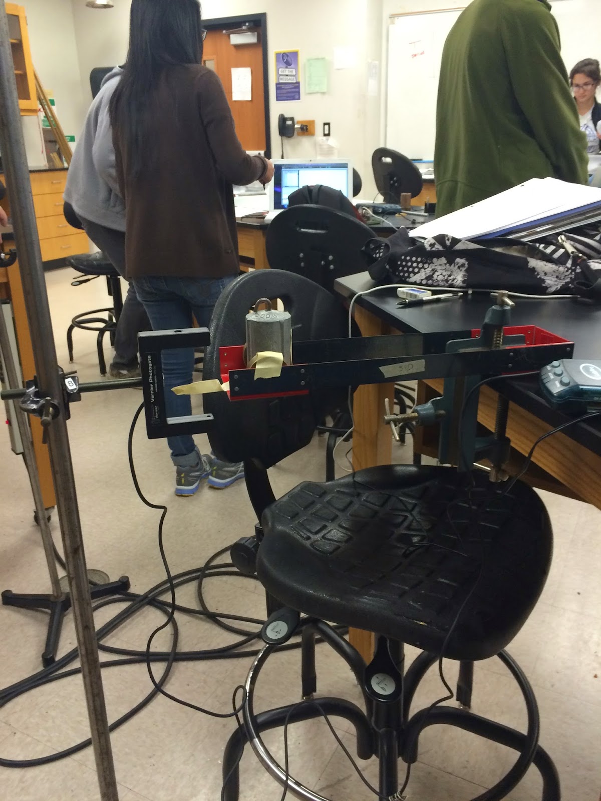
First of all, prepare some blocks which have different surface(means blocks have different coefficient of friction), Also prepare a pulley, a water cup, a empty cup, and a string:



mass of Normal block = 270.4g

mass of Red block = 126.3g

mass of each Blue block = 44.1g

mass of empty Cup = 2.9g










 And then, set up all of equipment such like the picture:























we are going to add water to the empty cup shown a little bit of a time until the block just starts to slip.

1) Put the Red block on the tabletop:   when add water to the empty cup until the cup has mass 49.9(mass of empty cup 2.9g + the mass of water 47g), the red block just starts to slip.

2) Put Red block on the tabletop and Put Normal block on  the top of Red block :   when add water to the empty cup until the cup has mass 119.5g (mass of empty cup 2.9g + the mass of water 116.6g), Two blocks just starts to slip.

3) Put Red block on the tabletop, Put Normal block on  the top of Red block, and put a Blue block on  the top of normal block:   when add water to the empty cup until the cup is mass 127.1g (mass of empty cup 2.9g + the mass of water 124.2), Three blocks just starts to slip.

Then put the measurements into Data Set:























There is a graph about Normal Force vs. Friction Force coming out:


















From this graph, we know the A is the coefficient of static friction μ(s) which means there is the coefficient of static friction μ(s) = 0.2985 between red block and tabletop.

Part 2 : Kinetic Friction

We model sliding, or "kinetic", friction as being proportional to normal force, and independent of the area or speed of the moving object. we write:
                                         f(kinetic) = μ(k)N
In our model, the kinetic friction force has a fixed value for a given N, regardless of the speed of the motion. We will use a Force sensor in this part of the lab.  Plug in a LabPro and connect it to the computer with the USB cable. Plug the force probe into the LabPro. Switch the force probe so that it reads in the 10-N range.  We are using the red block which mass is 126.3g to do this lab.

For run 1(red line), we were pulling the red block with a average force P(1)= 0.4457N

For run 2(blue line), we were pulling the red block and normal block is on its top with a average force P(2)= 1.236N

For last run(green line), we were pulling the red block and normal block and blue block on its top  with a average force P(3)= 1.386N



























Then, we plot the data into Data Set.
we will have a with graph of Normal Force vs. Friction Force.
the slope of the line is the coefficient of static friction μ(k) = 0.2758 between red block and tabletop.

Part 3 : Static Friction From A Sloped Surface.

Place a block on a horizontal surface. Slowly raise one end of the surface, tilting it until the block starts to slip. Use the angle at which slipping just begins to determine the coefficient of static friction μ(s) between the block and the surface.



1) Place a red block on a horizontal surface. when the red block starts to slip, the angle  θ is  19°. 
For this condition, we know the coefficient of static friction between the block and surface μ(s)  = tan 19° = 0.3443

2) Place a red block that there is a normal block on it top on a horizontal surface. when the red block starts to slip, the angle  θ is 12°
For this condition, we know the coefficient of static friction between the block and surface μ(s)  = tan 12° = 0.2126

3) Place a red block that there are a normal block and a blue block on it top on a horizontal surface. when the red block starts to slip, the angle  θ is 10°
For this condition, we know the coefficient of static friction between the block and surface μ(s)  = tan 10° = 0.1763

Part 4 : Kinetic Friction From Sliding a block down and incline.

With a motion detector at the top of an incline steep enough that a block will accelerate down the incline, measure the angle of the incline and the acceleration of the block and determine the coefficient of kinetic friction between the block and the surface from our measurements.

From the motion detector and the labPro, we have the graph of velocity vs. time.  And the slope is the acceleration a = 1.61 m/s^2


















we know the angle θ = 30°, the mass of red block = 126.3g, the acceleration = 1.61 m/s^2. then calculate the coefficient of kinetic friction between the block and surface μ(k) by Newton's law.

Part 5 : Predicting the acceleration of a two-mass system.

Using our coefficient of kinetic friction result from part 4 above, derive and expression for what the acceleration of the block would be if you used a hanging mass sufficiently heavy to accelerate the system as shown.

Predicting first, the predict of calculation is :

However, from the LabPro in the computer we have this graph of velocity vs. time about the block.

we could see the slope is 0.2983 m/s^2 from the picture. which means that the acceleration 0.2983 m/s^2 collected by the sensor is far from the acceleration 0.5813 m/s^2 we predicted. My partner and I may made some mistakes or wrote down some wrong data. that's why our predict is different the experimental.

Lab 5 : Modeling the fall of an object falling with air resistance

Part 1 : Determining the relationship between air resistance force and speed.

We have an expectation that air resistance force on a particular object depends on the object's speed, its shape, and the material it is moving through:
                                          F(resistance) = k * v^n 

First, we were going to the Design Technology building and do this lab by using video capture.

There is the linear portion of the position vs. time graph for 1 coffee filter falling from the balcony. we have a slope that means the acceleration = 1.049 m/s^2.

There is the linear portion of the position vs. time graph for 2 coffee filters falling from the balcony. we have a slope that means the acceleration = 1.219 m/s^2.

There is the linear portion of the position vs. time graph for 3 coffee filters falling from the balcony. we have a slope that means the acceleration = 1.686 m/s^2.


















There is the linear portion of the position vs. time graph for 4 coffee filters falling from the balcony. we have a slope that means the acceleration = 1.855 m/s^2.

There is the linear portion of the position vs. time graph for 5 coffee filters falling from the balcony. we have a slope that means the acceleration = 2.426 m/s^2.  

Then, plot all of accelerations and the mass of 1, 2, 3, 4, and 5 coffee filters to determine value for k and n.(like above two pictures)  And from this graph, we know the k = 0.01258, n = 1.497 .

Part 2 : Modeling  the fall of an object including air resistance.

We can use Excel to model the fall of an object with air resistance.








we start with the following conditions:

For my partner and I, we picked the mass of 3 coffee filters to test our measurements. we know the mass of 50 coffee filter = 46.3 g (for the mass of 1 coffee filter = 0.926 g).  after set up the k = 0.01258, m = 0.002778 kg(mass of 3 coffee filters), n = 1.497, gravity = 9.81 m/s^2, we choose the time interval △t= 0.01s.

From this data table, we could see that when t = 1.33s, the acceleration is almost equal to 0. for this moment, the velocity = 1.6759 m/s.    From the position vs. time graph for 3 coffee filters falling, we know the its velocity = 1.686 m/s.

Compare those two velocities, we could see that two velocities are so close which means our measurements are almost correct. And, the time interval 0.01s we chosen is the best to test the data.

Lab 4: Propagated uncertainty in measurements

Part 1 : Measuring the Density of Metal Cylinders

First of all, we have three different metals : Aluminum(Al), Copper(Cu), Iron Ferrum(Fe).
And we already measured all the data(like the picture, there are diameters, heights, and masses of metal) about three metals.


There are some formulas that we already know for calculating the density of metal, Therefore, we also need to calculate the propagated error in each of our density measurements because of Propagated uncertainty.















There are pictures about calculations :

There are calculations about the density and propagated of Al.  For this Al, our measurements are within the experimental uncertainty of the accepted values.

There are calculations about the density and propagated of Cu. For this Cu our measurements are within the experimental uncertainty of the accepted values.  

There are calculations about the density and propagated of Fe.For this Fe our measurements are within the experimental uncertainty of the accepted values. 

Part 2 : Determination of an unknown mass.

First, we need to get some spring scales, and an unknown mass. Set up two clamps onto the edge of a lab table as the picture, with a long rod in each.


Second, we measured the angles and record the scale readings, and we also estimated the uncertainty in your angle readings and scale readings.

There are some formulas by Newton's laws which is for calculating the mass of the unknown mass, And we also need to use our known uncertainties to calculate the propagated uncertainty in the calculated value(Need to know that whenever our calculus, our dθ has to be in radians, not degrees.).













There are calculations :

our measurements are within the experimental uncertainty of the accepted values. 

Then, use a different set of angles and a different hanging mass, do all steps again.

we got new data like the above picture:


For this new mass m2, there are calculations like the picture:

with a different set of angles and a different hanging mass, our measurements are still within the experimental uncertainty of the accepted values.

We could say that my partner and I are successful for this lab, because the propagation of uncertainty is the effect of variables' uncertainties on the uncertainty of a function based on them. 
However, all of our measurements are within the experimental uncertainty of the accepted values

Lab 3. Unconstant Acceleration

Today, we are going to find the relations between unconstant acceleration a and velocity v, and position x.

Example: There is a 5000kg elephant who has a constant velocity 25 m/s at the beginning. and the elephant has a rocket who is (1500 + 20t)kg on his back. Suddenly, the rocket starts to fire and gives 8000N to decrease the elephant.

There are calculation and equations :

From the equation of velocity,  we could know the graph of velocity:

Then, we can imagine △t is small enough,..

like the pictures, we could have some variables:
                                              when △t = 0.1s,

set t starts from 0.
t = t + △t

a = F/m = -400/(325 - t)      

△v = △a * △t = (a0 + a1)*△t/2        (a0 = -1.23 m/s^2)

v = v0 + △v = 25m/s + △v

v-avg = (v0 + v)/2

△x = v-avg * △t

x = x0 + △x



Open the excel, and input the data which we already know. and then we will have many data from t = 0s and time interval is 0.1s.  Here is the picture of data.

there is a v = 0 when t is between 19.6s and 19.7s,
right now, we can test our equations.
when t = 19.6s:

after calculated, we got almost same result with the data on excel.

For a unconstant acceleration problem, we can treat the graph of acceleration as a straight when we choose a time interval as small enough. then we could calculate anything we want.

2-Mar-2015 Free Fall Lab--determination of g and some statistics for analyzing data

The purpose of This lab is to examine the validity of the statement that in the absence of all other external forces except gravity, a falling body will accelerate at 9.8 m/s^2.

After professor has done the test with the equipment like picture 1.

(picture 1)

Professor gave us some series of dots on the paper corresponding to the position of the falling mass every 1/60^th of a second.(picture 2)

                                     (picture 2)

Place a two-meter stick next to the tape. Line up the 0-m mark with one of the dots and record the position of each dot as measured from the 0-cm mark. Then open Microsoft Excel and write down the data. (picture 3)

                                               (picture 3)

First cell  means time, I forget to enter TIME in cell A1.
X meas the distance between the dot and 0-m mark.
The third cell △x means the distance between the dot and next dot.
In cell D1, there is Mid-interval time (this gives the time for the middle of each 1/60^th second interval).
In the last cell, there is Mid-interval speed that comes from △x/(1/60).

we will have a line form the Mid-interval time/velocity graph(picture 4).
the equation is y = 9.60x + 0.69.

                                                                              (picture 4)
The slope is acceleration.  this acceleration 9.60 m/s^2 is our value of gravity.
After professor collected all of acceleration from other students in the class, we have a new data table(picture 5).

                                                                            (picture 5)

Then, we calculated a average g = 9.56 m/s^2.
The absolute difference is 9.56 - 9.8 = -0.24 m/s^2.
The relative difference is (absolute difference / 9.8)*100% = -2.45%

Different masses should have the same acceleration by freely falling-- gravity 9.8m/s^2. However, There were some errors. I think there was air friction. that is why we can not get the 9.8m/s^2.

28-Feb-2015: Find a relationship between mass and period for an inertial balance.

For this lab, we are going to find a relationship between mass and period for an inertial balance. the inertial balance is a device that is used to measure inertial mass by comparing objects's resistances to changes in their motion. 

First of all,  we need to set up the equipment like the picture1, 2, and 3.  

Use a C-clamp to secure the inertial balance to the table top. Put a thin piece of masking tape on the end of the inertial balance. Set up a photogate, and make sure the tape completely passes through the beam of the photogate when the balance is oscillating. Then set up the Labpro with a power adapter, USB cable, and plug adapter plugged into the DIG/SONIC input. 

(picture 1)

(picture 2)

(picture 3)

Next, Open the computer to choose Pendulum Timer.cmbl which is under Photogates Folder. Using the software to start data collection. Right now we can collect the data when you hit the collect button and pull back and release the inertial balance.

Record the period with no mass in the tray, then repeat the record, adding 100 grams each time until you have reached 800 grams in the tray. collecting two more data when we put calculator and phone in the tray. 

There is a Data Table(picture 4).

(picture 4)

we already know that the period is related to mass by some power-law type of equation:  

T = A(m + M)^n

After we take the natural logarithm of each side we get:

ln T = n ln(m + M) + ln A, which looks like y = mx + b.

That means that there is a beautiful straight-line if we have right data.

(picture 5)

Fortunately, we almost get a straight-line like picture 5 and 6, and we also get a straight-line equation. From this equation, we know A, M, and n. 

(picture 6)

Then, Using the different M to test the minimum of lnA and lnT and maximum of lnA and lnT. Now we have min-equation and max-equation.

plug in the data of calculator to each of equations like picture 7.

(picture 7)

plug in the data of phone to each of equations like picture 8.

(picture 8)

From those two calculations, we know the first calculation is right. because the mass of calculator is between the two masses we calculated. However, there was some errors in second calculation. the mass of phone(0.130kg) is not between the two masses we calculated. We may made some mistake during the data collection.